If you’re interested in data science, the Jupyter Notebook is an incredibly useful tool for developing and presenting projects interactively. This tutorial will walk you through the process of using Jupyter Notebooks for data science projects on your desktops, laptops or virtual machines.
Table of Contents
About Jupyter Notebook
Notebooks are versatile document that combines code and its output, along with visualizations, narrative text, mathematical equations, and other rich media. They allow you to run code, display the output, and add explanations, formulas, charts, and more. Essentially, notebooks provide a way to make your work more transparent, understandable, repeatable, and shareable in one single document.
If you’re working with data, Notebooks can be a game-changer. They’ve become an essential part of the data science workflow in companies worldwide thanks to their ability to speed up workflows, simplify communication, and make it easy to share results.
As part of the open-source Project Jupyter, Jupyter Notebooks are completely free. You can download the software alone or as part of the Anaconda data science toolkit.
While Jupyter Notebooks support various programming languages, this article will concentrate on Python, which is widely used.
Following this article
First, we will cover installing Jupyter Notebook in Linux and Windows. Then we will talk about the various user interfaces and keyboard shortcuts for interactive use.
Installing Jupyter
If you’re just starting out with Jupyter Notebooks, consider installing Anaconda to get up and running quickly. Anaconda is a top Python distribution for data science and includes many of the most popular libraries and tools pre-installed, such as NumPy, pandas, and Matplotlib. It’s arguably the best way to start.
To install Anaconda, you can refer to our guide in this tutorial.
If you prefer to only use Jupyter and not a whole lot of packages, you can simply open a command prompt and run the following to install Jupyter. You can also read this guide to install Jupyter.
pip3 install jupyter
Creating Your First Notebook
In this section, you’ll learn how to run and save notebooks, understand their structure, and navigate the interface. We’ll also go over key terminology to help you confidently use Jupyter Notebooks and prepare for the next section. The subsequent section will walk us through a data analysis example, putting everything we’ve learned into practice.
Running Jupyter
Jupyter Notebook runs on a browser via a local server installed by Anaconda or Jupyter. Hence, make sure you have a browser installed such as Firefox or Google Chrome or Edge.
On Windows, go to the start menu and launch Anaconda. From the Anaconda panel, click on Jupyter Notebook.
If you have installed only Jupyter using pip, then from the command prompt, run the following to launch Jupyter Notebook.
jupyter notebook
Upon successful run, you should see the default browser opens up as the following. This means your Jupyter Notebook is running fine.

This page that opened above is not a notebook yet. It’s actually the Notebook Dashboard, designed to help you manage your Jupyter Notebooks. Consider it your launchpad for exploring, editing, and creating notebooks.
Keep in mind that the dashboard only provides access to files and sub-folders located within Jupyter’s startup directory, which is where Jupyter or Anaconda is installed. For example, you can run the command "jupyter notebook" by traversing to any directory from the command line. The page will open on that current working directory.
You can also use the following command to launch Notebooks with a custom working directory.
jupyter notebook --notebook-dir="/home/arindam/Downloads/"

When you open Jupyter Notebook in your browser, you may notice that the URL for the dashboard starts with "https://localhost:8888/tree". Localhost means that the content is being served from your own computer, i.e. built-in jupyter server. Jupyter’s Notebooks and Dashboards are web applications, and Jupyter runs a local Python server to serve these apps to your web browser. This makes it platform-independent and easier to share on the web.
The dashboard’s interface is mostly self-explanatory, which we will cover in the later section below. Select a folder from the list of folders and select new > Python 3 from the top menu. This will create your first Notebook.

Each notebook opens in the new tab of your browser. It helps when you work with multiple notebooks simultaneously. If you go back to the dashboard, you should see a new file is created named Untitled.ipynb. The green text tells that it is running.
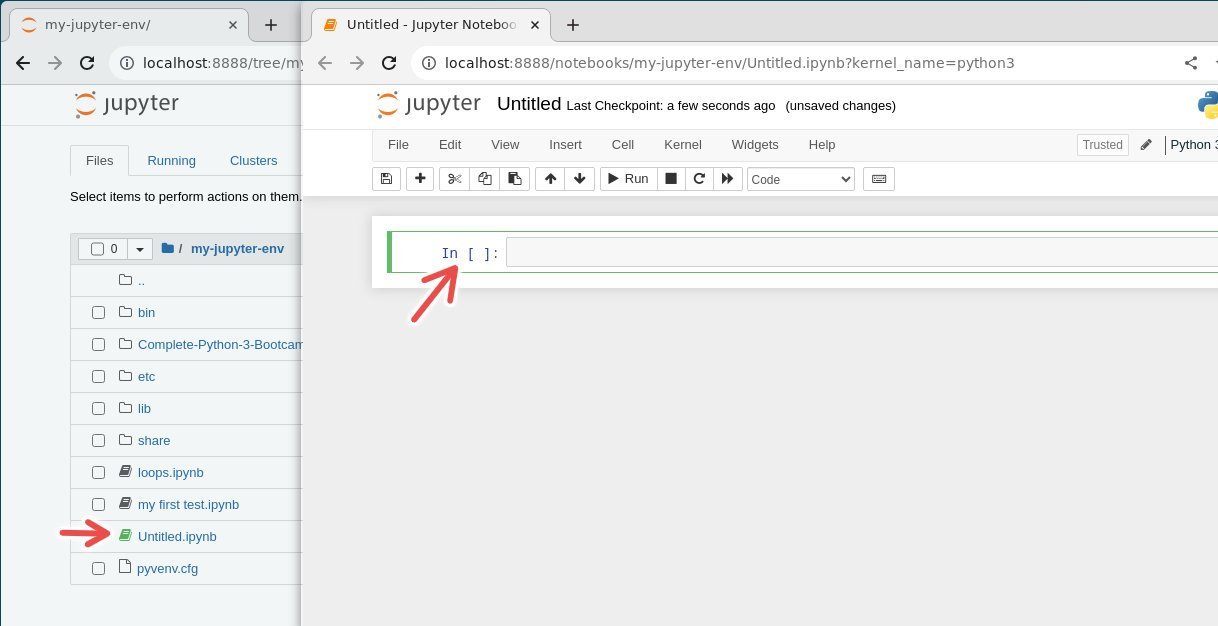
What is an ipynb File?
When you create a new notebook, a new file is created having an extension of ipynb. This file is essentially a text file that uses JSON format to describe the contents of your notebook. It includes each cell and its contents, along with any image attachments that have been converted into text strings and some metadata. You can view your notebook’s contents by selecting “Edit” from the dashboard controls, but editing the metadata yourself is not recommended.
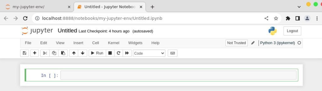
The Notebook Interface
When you open the .ipynb file, the notebook interfaces open up for that file. You can look around and get a feel of the user interfaces, menus and commands.
You can click on each of the menu items to see what are the available options. All the menu items are basically notebook commands which can be accessible using the small “keyboard” icon.
Two key menu items which you should know about here are “kernel” and “cell”.
- A kernel is a computational engine that runs code in a notebook.
- A cell in the notebook contains text or code to be executed.
Cells
Cells are the backbone of any Notebook. It may contain your code or any markdown text. So, the Code cell contains codes which can be executed by the Python kernel. When you run the code, the output is displayed below the cell that generated it.
A markdown cell contains formatted texts and displays its output at the same place when you run the markdown cell. Markdown cells may contain headings such as H1, H2 etc. or any basic text formatting. Hence, you can also use Notebooks to prepare code documentation. It’s very useful in that use case.
Let’s try out a basic Python statement in a code cell. Type the following in your sample notebook file and click on the Run button in the toolbar. You can also press SHIFT+ENTER or LEFT CTRL+ENTER to run it.
print('hello!')

When you run it, the output is displayed just below the cell and the label In [ ] changes to In [1].
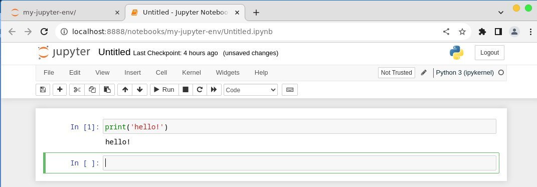
The “In” denotes “Input” and the number represents the “when” in time the cell executed. If you run the cell again, the label changes to In [2].

When a cell is executing the label shows as In [*]. Also, the markdown cells do not have any labels.
A few shortcuts
Although the Notebook interface has menu items which you can use, it’s productive and efficient to use keyboard shortcuts.
For example, to quickly run a cell you can press SHIFT+ENTER or LEFT CTRL+ENTER – instead of clicking the Run button from the menu.
Similarly, here is a quick table for various functions of the Jupyter Notebook:
| Function | Keyboard shortcut |
| Scroll up or down to traverse the cell | Use Up or Down keys |
| Toggle command (blue) and edit (green) mode | Escape or Enter |
| Insert new cell above | Press A |
| Insert new cell below | Press B |
| Convert a cell to markdown | Press M |
| Convert a cell to code cell | Press Y |
| Delete the cell | Press D + D (press D twice) |
| Undo the deletion | Press Z |
| Select multiple cells | Hold SHIFT and UP / DOWN arrow key |
Markdown cells
You probably know about Markdown which is easy to learn and uses formatting methods for plain texts. It’s similar to HTML but the tags are different. You can also use Jupyter Notebook for creating nice documentation using its markdown cells.
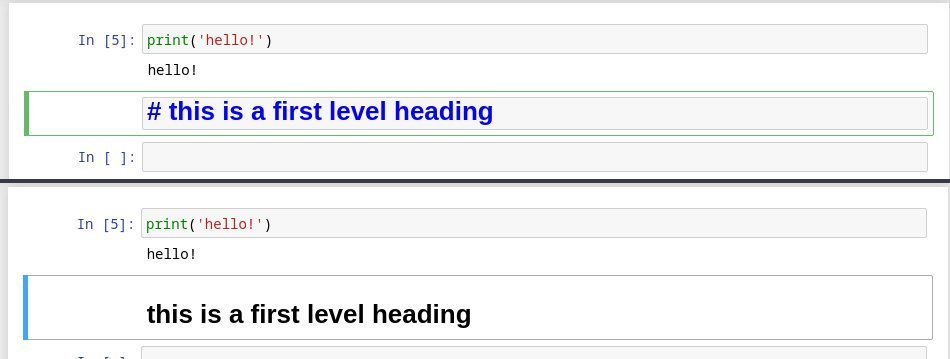
For example, a single # followed by a line can make a first-level heading i.e. H1 tag in HTML.
# This is a first level heading
Here’s an example of a more complex markdown example which you can try in Jupyter Notebook. Remember, these need to be added to the markdown cells (press M).
# This is first level heading h1

## This is second level heading h2

A simple line of text.
A **bold** word
Another __bold__ word
This is *italics* or _italics_

* A list item
* Another list item

1. List with numbers
2. Another item

This is a hyperlink [debugpoint.com](https://www.debugpoint.com)

The following is a code block:
```
print('hello')
print('world')
```
And when you run it, it shows in proper formatting.

Kernels and execution flow
When you create a Notebook, and run a code – the code is executed within the scope of that notebook kernel. The state of your variables and values persists between cells. That means the values and state of variables scope is the entire document and not the individual cells.
For example, if you import any library in one cell, you can use the functions of that library in another cell. Here’s a quick example where we imported numpy library and did an sqrt to a number.
import numpy as np
def find_sq_root(x):
    return np.sqrt(x)
You can put the above in one cell and call the function in another cell.
find_sq_root(44)
As you can see the the defined function is available throughout the document and not to individual cells.

The execution flow of a Notebook from top to bottom. However, you can select any cell at any time and execute it. While doing so, remember that the variable and function scope is the entire document. Hence be cautious while writing programs.
The number beside In shows the execution order. It increments in each execution of cells. It reflects the order of cell execution in the Kernel in the scope of that document.
For example, in the below example, you can see the two print statements are executed and then the square root function. Hence the print statements are showing In [6] and In [7] and so on.

At any time, if you lose track of execution and want to reset the entire document, you can do so using the Kernel options.
- To restart the Kernel and clear all variables: Use Restart
- If you want to restart, clear all variables and clean all outputs: Use Restart and clear output
- Lastly, to restart and execute everything: Use Restart and Run all
If you run into race conditions or infinite loops, you can use the Interrupt option to stop the execution.

Other language support in Kernel
Jupyter Notebooks are versatile to support many languages, not only Python. For example, you can install and run C, R, Julia, Java and other popular programming languages.
You need to install the proper kernel for those using pip and select the Kernel from the Kernel > Change Kernel option.
You can learn more about additional support here.
Saving your Notebooks
Remember to save your notebooks periodically from the menu. Or you can press CTRL+S to do manual save and checkpoint.
Once you complete your work, you should use the File > Close and Halt option from the menu. This ensures the executions shut down the Kernel of the respective notebook and close the browser tabs.
You can also download your Notebook in HTML, PDF and other formats using the File menu.
Before you download and save, ensure to clean your work using the below options.
- Click on “Cell > All Output > Clear”
- Click on “Kernel > Restart & Run All”
- Wait for all execution complete.
Wrapping Up
I hope you get a basic understanding of Jupyter Notebook in this tutorial. From the installation steps to creating your first Notebook. You also learned the shortcuts, Kernels, cells and scope of execution.
You can start exploring more as you go with official documentations.
Cheers.


